Mapping Acoustic Similarity

The idea of similarity is a common component of recommender systems. When deciding what content to recommend to a user, algorithms can draw on different elements of similarity:
- Users, based on the similarity of content they consume
- Users, based on the similarity of characteristics (e.g. age, geography)
- Content, based on it being consumed in similar patterns
- Content, based on the similarity of characteristics (e.g. tempo, instrumentation)
When it comes to music, the characteristics which can be used to model the similarity between items is extensive. Libraries such as Essentia, for example, include hundreds of candidate features which can be extracted from audio files. For each feature, different statistics (e.g. measures of central tendency or dispersion) can be used to summarise how that feature is reflected in a content item.
Our previous research into Australian art music identified a set of 13 acoustic features to use in calculating the similarity between items. We arrived at this set of features by first surveying Australian composers about how similar they consider their own music is to that of other composers.
We then tested tens of thousands of different combinations of acoustic features to identify which set was best at reproducing the similarities observed in our survey. The resulting set of features is shown in the table below.
| Essentia Category | Acoustic Feature |
|---|---|
| Low Level | ERB Bands Flatness (Mean) |
| ERB Bands Kurtosis (Standard Deviation) | |
| ERB Bands Spread (Standard Deviation) | |
| Mel Frequency Cepstrum Coefficient 1 (Mean) | |
| Mel Frequency Cepstrum Coefficient 2 (Mean) | |
| Zero-crossing Rate (Mean Absolute Difference) | |
| Rhythm | Beats per Minute (BPM) |
| Second-highest peak value of the BPM histogram | |
| Sound Envelope | Log Attack Time |
| Temporal spread | |
| Tonal | Crest of the harmonic pitch class profile (HPCP) vector (Standard Deviation) |
| Shanon entropy of the HPCP vector (Mean Absolute Difference) | |
| Strength of key estimation |
Given a corpus of recordings, these acoustic features can then be used to generate a dissimilarity matrix. Rather than individual songs, dissimilarities can be measured between the overall output of individual artists, resulting in a matrix which represents how similar (or dissimilar) each musical artist is from every other artist in the corpus.
In our research we analysed a library of 15,000 recordings by 300 Australian composers to produce a dissimilarity matrix based on the Mahalanobis distances between each composer using our 13 acoustic feature set.
library(Rfast) # for pooled.cov() pooled covariance calculation
library(biotools) # for D2.dist() Mahalanobis distance calculation

# audioFeatures contains the audio descriptors for a corpus recordings, together with the name of each recording’s composer/artist
audioFeatures <- tibble(descriptor1 = c(…), descriptor2 = c(…), … descriptor13 = c(), composer = c())

# calculate the mean for each composer across each audio descriptor
composerMeans <- audioFeatures %>% group_by(composer) %>% summarise_all(mean)

# calculate the pooled covariance representing the weighted average of covariance among the audio descriptors for each composer
pooledCovariance <- pooled.cov(as.matrix(audioFeatures %>% dplyr::select(-composer)),factor(audioFeatures$composer))

# calculate the Mahalanobis distance between each composer
dissimilarityMatrix <- as.matrix(D2.dist(composerMeans %>% dplyr::select(-composer), pooledCovariance))
colnames(dissimilarityMatrix) <- unique(audioFeatures$composer)
rownames(dissimilarityMatrix) <- unique(audioFeatures$composer)
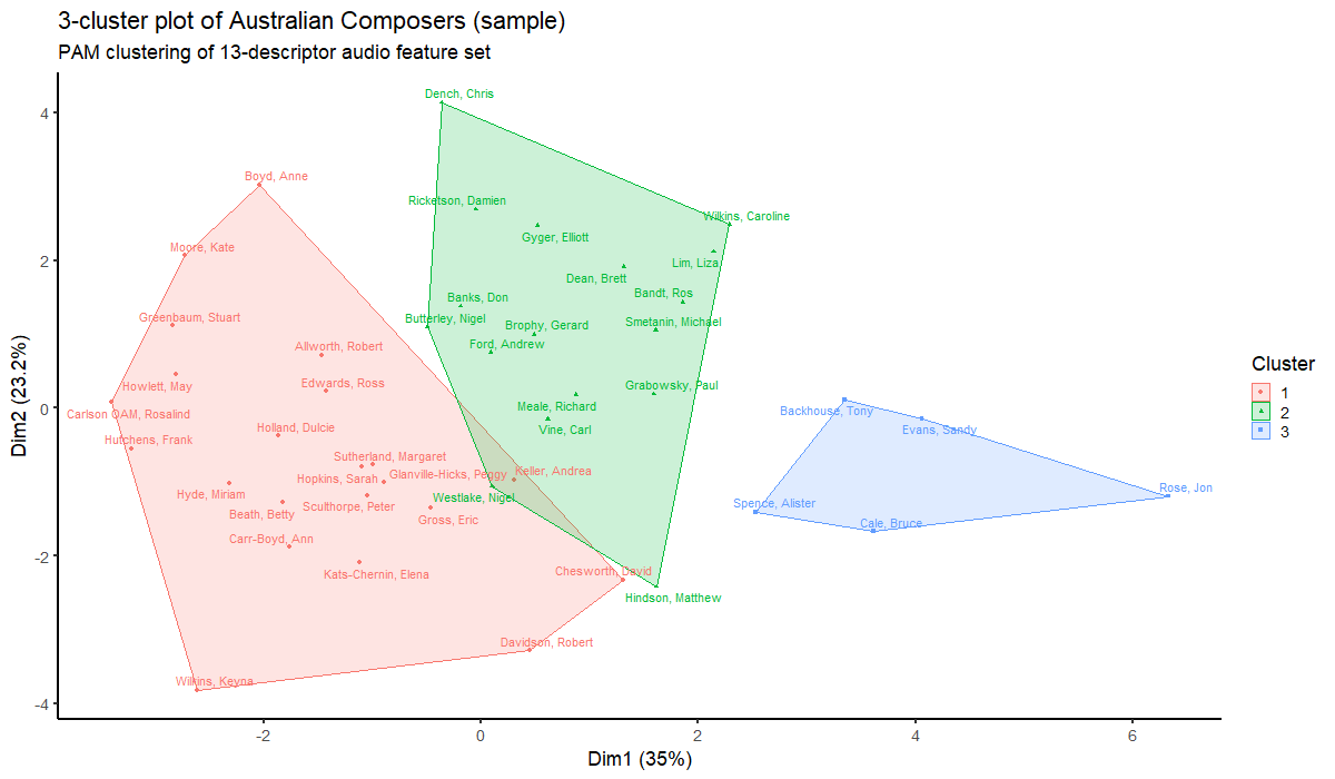
Having obtained a dissimilarity matrix based on acoustic features, we can then use this to produce various projections of the acoustic space of Australian art music. Clustering, using partitioning around medoids (PAM), for instance, shows three groups of composers. Composers in Cluster 1 reflect those who operate in an idiom of traditional tonality; Cluster 2 brings together those whose work exhibits more modernist stylistic influences; while Cluster 3 includes those who operate predominantly in jazz-influenced idioms.
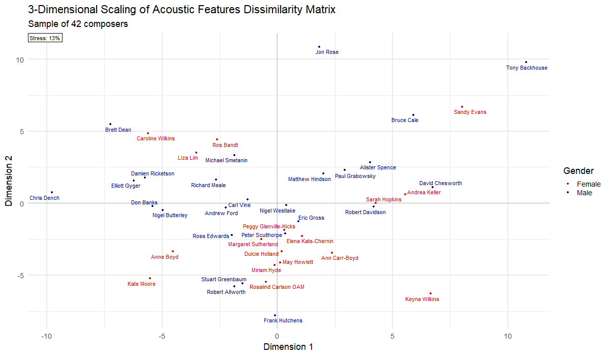
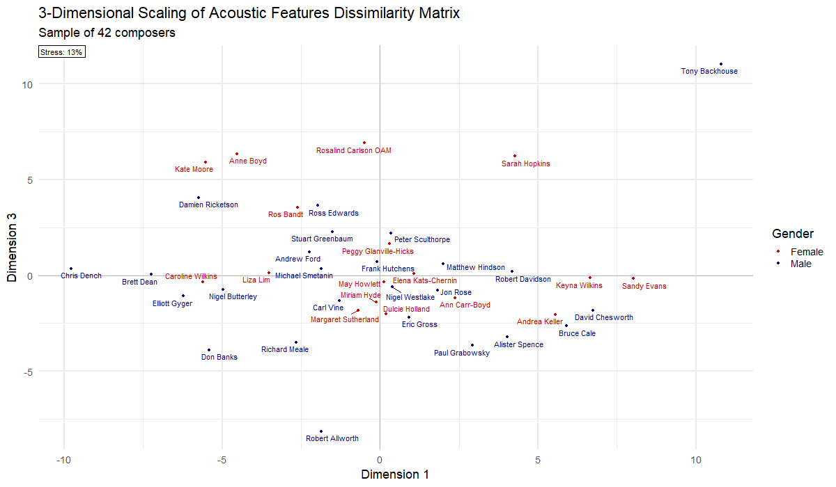
Alternatively, the dissimilarity matrix can be visualised using multi-dimensional scaling. This plots the relative location of individual composers on a series of n dimensions. The spread of composers across each dimension can point to latent organising principles of a field of practice. In the case of Australian art music, we observed three dimensions:
| Dimension | Negative | Positive |
|---|---|---|
| 1 | Modernism | Jazz and minimalism |
| 2 | Traditional | Experimental |
| 3 | Serialism | Spiritualism and nature |
The approaches above demonstrate some of the ways in which distances between musical artists can be calculated and then used to map a broader space of musical activity to uncover aspects of how that space is structured and organised.